Introduction to CasaXPS (complete PDF of this mini HowTo).
I. General
1. Open vms file in CasaXPS, double click the .vms file, or in Casa, File, Open
2. The first time you use CasaXPS enter the User Name and License in order to be able to save files.
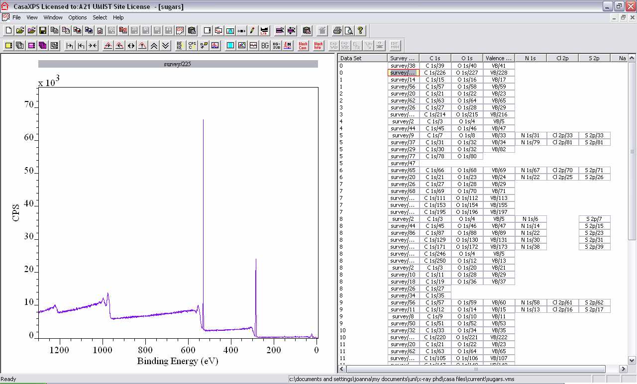
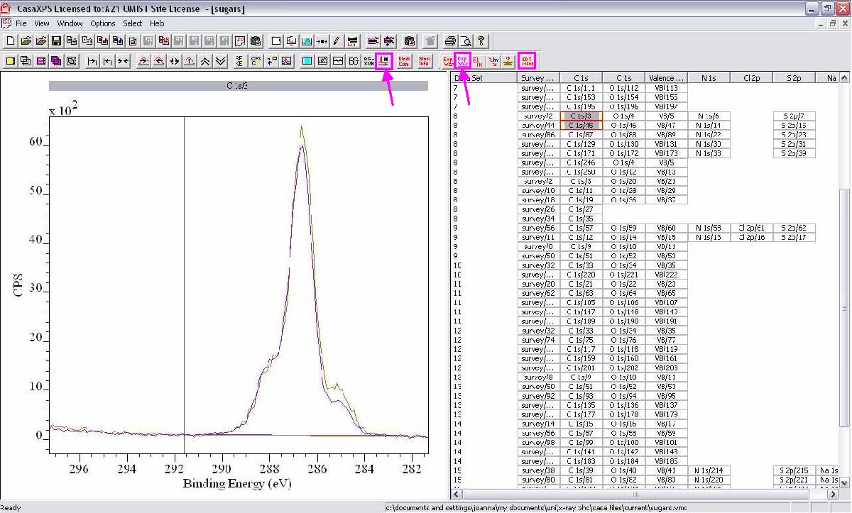
3. Casa XPS layout is divided into 2 sections:
- The left-hand side displays the spectra.
- The right-hand side lists the data blocks.
3. General mouse actions in CasaXPS:
- Left double-click: Select data block
- Shift then left click: Select all blocks between 1st and last selected block
- Ctrl then left click: Select the 1st block and another block
- Left click and drag a box: Magnifies the area within the box (double-headed arrow zooms out)
- Right click in data block side: Copy selected blocks
- Right click in spectra side: Propagate the specified quantification (regions, components, processing, annotation) from one spectra to others
- Left click within the spectrum: Allows the Options menu to be accessed.
II. The Options menu:
1. Page layout – for choosing how many spectra are displayed at a time.
2. Tile display – for choosing what parameters are displayed, font size, colours, etc.
3. Quantify – for setting up and checking the regions and peak components.
4. Elements – for identifying and quantifying the wide survey spectra.
5. Processing – for calibrating the spectra.
6. Annotation – for displaying the region and component % values, FWHM, etc.
When editing data in the Quantify, Regions or Components tabs, ensure Enter is pressed to retain the changes.
III. Identifying and quantifying the elements present
1. Double-click on a Wide (survey) data block to display the spectra, then click in the spectra.
2. Options, Elements, Periodic Table, Find Peaks to locate the elemental peaks.
3. Only the main photoemission peak is chosen per element (e.g. for C, O, and N the 1s; for Cl, S the 2p, etc.)
4. Check that all the expected elements are selected, and that no obvious peaks have been omitted.
5. Click Create Regions to create the quantification, then click Clear All Elements. The default background is ‘Linear’, and the Relative Sensitivity Factors (RSF) are entered automatically.

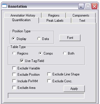
6. Options, Annotation, Quantification, ensure Display, Comps, and Use Tag Field are selected, then click Apply. The atomic % of each element is displayed on the spectrum. Annotation History records the annotation applied to each data block.
7. Click within the spectrum, press the double-headed arrow on the toolbar, then press the lefthand arrow to zoom in on each region in turn. Check that the region background looks right – the left side should always be slightly higher than the right, and the background line should neatly bridge the gap underneath the peak.
8. If the background is not quite right, Options, Quantify, Regions. This box shows the quantification carried out, including the element photoemission level, RSF, and background type. When on the Regions tab, there will be a pale blue region shown on the spectrum, with two edge lines either side. To modify the Region, click and drag either of these edges.

IV. Analysing chemical environments
1. Select the high resolution element data block, and activate the spectrum on the left. If needed, zoom in by drawing a box around the peak.
2. Options, Annotation, Quantification, ensure Data and Comps are selected, then Apply.
3. Options, Quantify, Regions, click Create. Drag the edges of the region created to either side of the photoemission peak, in a similar manner to the survey spectra. Check the RSF and background type (change if required) and change the Tag to read NoTag.
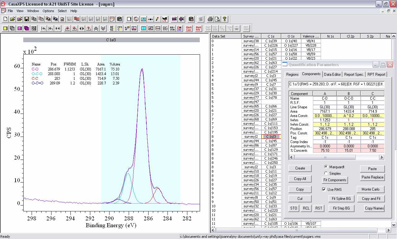
4. Options, Quantify, Components. In the same box, switch to the Components tab and click Create. Either click Fit Components a few times (three should be sufficient) or if it obvious there is more than one peak within the overall shape, more than one component can be created then the Fit Components button pressed.
5. The program only attempts to produce a good fit to the overall shape of the data. It has no knowledge of the chemistry or chemical environments present. It is up to the user to ensure their fitting and numbers of peaks have a meaningful, scientific explanation. Good references for common ranges for chemical shifts for different environments/bonding/oxidation state are the Appendices of the The XPS of Polymers Database, and NIST (http://srdata.nist.gov/xps/).
6. With an idea of how many peak components are required for your compound (based on the chemical structure), try and fit the spectra.
i. Keep in mind the FWHM should be fairly similar per elemental region [typical values are 1-1.2 eV for C1s and N1s, 1-1.4 eV for O1s].
ii. Constraints can be applied to the Area, FWHM, and position, and can be for a range (FWHM Constraint as 1, 1.2 would limit FWHM to within 1 and 1.2 eV) or relative to another component (for example, if the Area Constraint of component B is written
as A*0.5, then the Area will be ½ that of component A).
iii. FWHM Constraints are used to ensure the components do not get too wide, Position Constraints are used when you have an idea of the approximate position of the component, or do not want it to move too far, and Area Constraints are used when
fitting to the stoichiometry of a chemical structure.
iv. A component can be moved manually by left clicking and dragging up/down for intensity or left/right for FWHM while the Components tab is open. Holding down the Shift key while dragging allows one variable to be altered without the other.
v. Components can be renamed to represent their chemical environment, etc., by changing the Name in the Components tab.
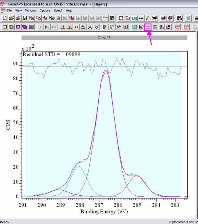
vi. The icon with the Residual icon displays the standard residual between the fit and the experimental data. Generally, the closer the value to 1 and less noisy the residual, the better the fit. A good visual check is the correspondence between the experimental data and the fitted peak envelope.
V. Referencing
1. Insulating samples accumulate a positive charge across the surface as the electrons are ejected. To compensate for this, low energy electrons are directed towards the sample via the charge neutralizer. The neutralizer often slightly overcompensates, generating a slight negative charge, resulting in photoemission peaks that are slightly shifted to low binding energy. Photoemission peaks must be adjusted to account for this for comparisons of binding energy to be viable.
2. For organic samples, the common method is referencing to adventitious hydrocarbon contamination at 285 eV (present in small quantities on all samples exposed to air), representing the chemical environment C–C. Hydrocarbon contamination will often lead to slightly increased C% and C–C intensity in spectra.
3. The hydrocarbon contamination peak may often be obscured by other peaks (C–C bonds may naturally be present); if C=C bonds are present, samples are often referenced to them instead as they occur at lower binding energy of 284.8 eV, making it easier to fit to.
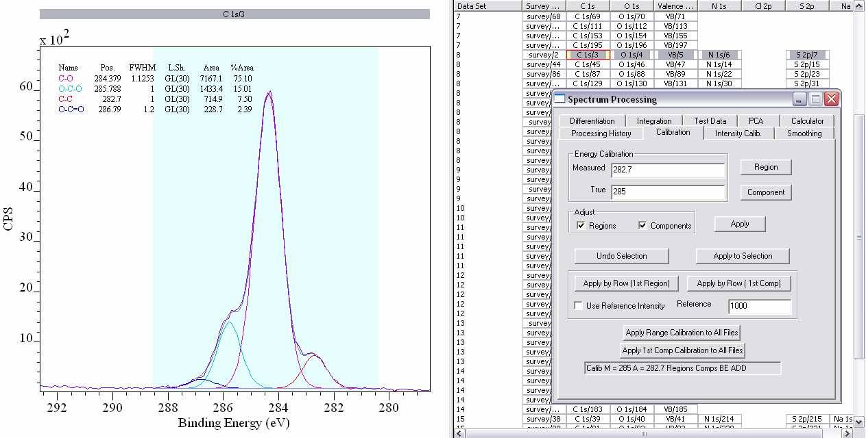
4. To reference spectra, Options, Processing, Calibration.
i. Either type in the experimentally Measured binding energy or draw a box on the spectra with the right-hand edge at the measured value.
ii. Type in the value to be shifted to in the True box (for example, Measured 282.7, True 285 eV to reference to adventitious hydrocarbon contamination 285 eV), and tick Regions and Components.
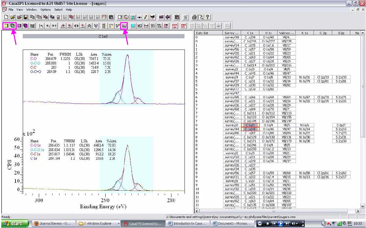
iii. To apply the calibration to all of the high resolution spectra in a row (for a single sample), click Apply to Selection.
VI. Survey and high resolution spectra:
1. The survey and high resolution data can be used together to give the atomic % of each of the components out of the total for that element. Select the survey data block, then Ctrl click the desired high resolution element block. If the annotation has been set up correctly as outlined previously, the survey spectrum will show the atomic % per component.
2. Spectra can be overlayed by selecting the desired data blocks and clicking the Overlay icon (second from the left, bottom row). Selecting the Offset icon changes the between overlayed and vertically offset spectra. Choosing the first icon on the left sets up the spectra to allow the Page Display option to be used to display multiple spectra horizontally or vertically.
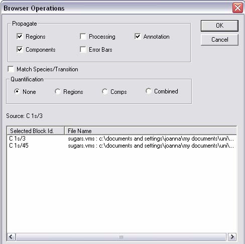
3. Regions, components, annotation, or processing can be propagated (copied) to other spectra by right clicking in the spectra side of the window. Propagating regions and components is especially useful for a series of similar compounds where you
want to fit the same components without having to do each one separately. After propagating, refine the regions and press Fit Components for the components.
4. Spectra can be normalised by overlaying the spectra and then selecting the Normalise icon. Holding down the Shift key and left clicking allows the position at which the spectra are normalized to be changed (represented by the black line).
5. The Block com icon contains the experimental acquisition details.
6. To copy data blocks to other windows/files, select the required blocks, go to the where the data is to be copied to, then click the Paste icon.
7. To number samples, select the required data blocks, and click the Exp Var icon, typing in the desired number for the Exp Variable Value.
8. To change the sample ID, click the Edit Mode icon select the data blocks and click the ?Edit Sample ID icon. Ensure only Update Sample ID is ticked, then type in the sample identity. Click OK, then Yes when prompted ‘Would you like to use the VAMAS ID instead?’.
VII. Exporting to Excel
1. Options, Quantify, Report Spec. Select whether data for Regions, Components, or both are required. The data for the selected data blocks is shown on screen. The Copy icon may then be used to copy the data into Excel.
VIII. Useful links
NIST database: http://srdata.nist.gov/xps/
XPS International: http://www.xpsdata.com/
CasaXPS: http://www.casaxps.com
Manuals: http://www.casaxps.com/ebooks/ebooks.htm
Updates: http://www.casaxps.com/help_manual/manual_updates/
RSF library for Kratos instruments
For data collected using Kratos instruments, the Kratos RSF reference library should be used. The default RSF library in CasaXPS is Schofield.
Download the Kratos reference library from http://www.casaxps.com/kratos/
To load the library, go to Element library > Input file > Browse > select the downloaded file > load
Keep the file type as CasaXPS lib
© Joanna S. Stevens 2011/2 The University of Manchester